Raytracing is an elegant mathematical framework for physically realistic light transport.
However, to appreciate the elegance of ray tracing, we must first understand how traditional rendering works.
Traditional rendering uses a technique called rasterization which maps the scene geometry to pixels by asking “how much of this object can be seen by this pixel”. It uses shaders to determine how the geometry looks - things such as color, specular highlights, and reflections.
Now, it’s remarkable that shaders work in the first place. It’s all smoke and mirrors relying on clever algorithms which imitate a photo-realistic look.
However, since rasterization relies on hacks, there are some light behavior which we cannot capture, or is difficult to capture using this technique.
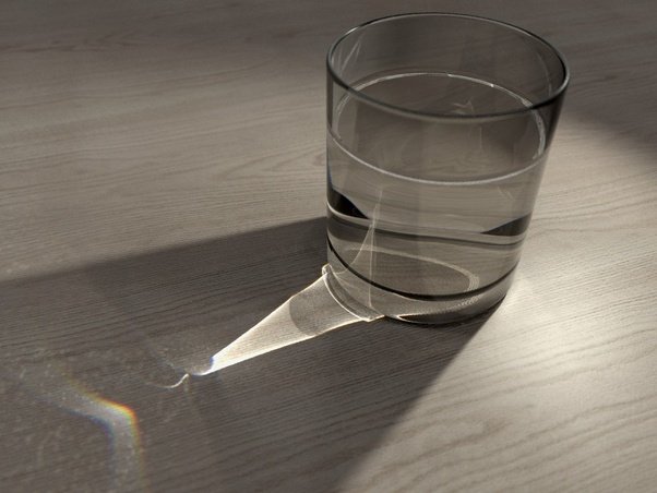
For example, you cannot accurately simulate complex scenes with transparency using rasterization. Furthermore, since most shader models such as the Lambert diffuse shader assume infinitely thin materials making simulating subsurface scattering difficult.
Finally, in real life, shadows are generally soft because light is reflected causing indirect illumination. However, rasterized rendering isn’t able to accurately simulate this in an efficient manner, so one of the techniques used to simulate indirect illumination is just to add a base amount of light to everything, so shadows will appear soft. Never mind that this trick violates conservation of energy and thereby the first law of thermodynamics.
Ray tracing solves all this using a simple and elegant mathematical framework.
Instead of trying to work out which pixels an object corresponds to, raytracing flips rendering on its head.
Raytracing works by shooting ‘rays’ from the camera and tracing which objects they hit, hence the name raytracing.
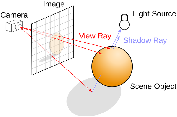
When a ray hits an object, it can simulate how light really would behave when interacting with the material.
Light can do two things when interacting with a material, it can be reflected, and it can be absorbed. And due to conservation of energy, the total energy going into the system must be equal to the energy going out.
Using just these three principles, we can simulate light with arbitrary precision. In fact, it’s virtually impossible to tell the difference between real life and simulation.
As an aside, astute readers may notice that in effect I’m not talking about raytracing, but instead an extension to raytracing called path tracing.
Path tracing gives extra effects - notably transmission - for free.
This is entirely on purpose as the general idea of simulating light rays is the same, and there’s no point in further complicating the details. Both raytracing and pathtracing share the same idea or method of thinking about light.
With raytracing, we get all effects we had to use complex tricks to recover with rasterization for free.
The downside of raytracing is that it’s computationally much more expensive than rasterization, and can only be calculated in real time (within 16ms) by the fastest graphics processors, and that only works for specific parts of a scene.
So it’s mostly used in prerendered scenes such as movies.
The math - the rendering equation
While we can talk all day about how raytracing works qualitatively, I don’t think it does it justice showing just how elegant it is.
I genuinely believe you have to see the math to truly appreciate it. While I’ve done my best to make the math accessible, if you’re scared of integrals - especially unsolvable integrals, you may want to skip the rest of this answer.
If we wanted to be 100% authentic to the physical world, we would simulate light by solving the Maxwell equations which precisely describe how electromagnetic waves behave, but that’s not practical as we’d never be able to actually compute anything.
Instead, we think of light as rays using the rendering equation. At the heart of the rendering equation lies conservation of energy.
It states that the outgoing light ($L_{0}$) is the sum, or integral, of the emitted light ($L_{e}$) and the reflected light ($L_{i}$).
Mathematically, we can write the rendering equation as
$$L_{0}\left(\mathbf{x}, \omega_{0}, \lambda, t\right)=L_{e}\left(\mathbf{x}, \omega_{0}, \lambda, t\right)+\int_{\Omega} f_{r}\left(\mathbf{x}, \omega_{\mathbf{i}}, \omega_{0}, \lambda, t\right) L_{\mathbf{i}}\left(\mathbf{x}, \omega_{\mathbf{i}}, \lambda, t\right)\left(\omega_{\mathbf{i}} \cdot \mathbf{n}\right) \mathrm{d} \omega_{\mathbf{i}}.$$
If you haven’t seen this before, it probably looks super scary, but fret not, it’s actually much simpler than it looks.
- $x,\omega$ are used to describe the position and direction of something.
- $n$ is standard notation for the surface normal at $x$.
- $\lambda$ is the wavelength of the light.
- $t$ is the time.
- $L_{0}$ is the outgoing light.
- $L_{e}$ is the emitted light.
- $L_{i}$ is the incoming light.
- $\Omega$ is the surface of a unit hemisphere centered around $n$.
- $f_r$ is the bidirectional reflectance distribution function (BRDF) - it describes the proportion of light reflected from $\omega_i$ to $\omega_0$.
Furthermore, the term $(\omega_i \cdot n)$ is there because less light is absorbed if the surface is leaning away from the light source. This is also why solar cells are angled such that they point towards the sun.
In summary, the rendering equation says:
The outgoing light at this location and in that direction is equal to the light emitted at this location in that direction plus the sum of the incoming light in all directions in the half hemisphere corrected for material and angle.
There’s just one problem.
We cannot solve the integral in the rendering equation.
At least, not analytically. If we look at the equation, we see that the extant radiance of a point $x$ depends on the incoming radiance of every other point, which also depends on $x$.
This is where raytracing comes in as it provides an algorithm for approximating the rendering equation.
A note about BRDFs
BRDFs are used in both rasterization approaches such as global illumination, and raytracing.
The BRDF explains how light is reflected from opaque materials. It’s what determines if the material looks like plastic, metal, or leather.
A simple diffuse BRDF, for example a soft plastic, might be
$$f_{r}\left(\mathbf{x}, \omega_{\mathbf{i}}, \omega_{0}, \lambda, t\right)=\frac{1}{\pi}$$
which collects radiance from all directions on the hemisphere with equal probability.
A specular BRDF, for example a mirror, on the other hand only collects radiance in the reflected direction
$$f_{r}\left(\mathbf{x}, \omega_{\mathbf{i}}, \omega_{0}, \lambda, t\right)=\left\{\begin{array}{c}{1, \text { for the reflected direction }} \\ {0, \text { for everywhere else }}\end{array}\right.$$
A glossy surface like a metal is a combination of the two.
For the BRDF to be physically valid, the function needs to satisfy a few additional properties:
- Positivity (no black bodies): $f_r(\omega_i, \omega_o)\geq 0$
- Helmholtz reciprocity: $f_r(\omega_i, \omega_o)=f_r(\omega_o, \omega_i)$
- Conservation of energy: $\forall \omega_o, \int_\Omega f_r(\omega_i,\omega_o) (n\cdot \omega_i) \mathrm{d}\omega_i \leq 1$
But what about glass?
Until now, we’ve only considered opaque materials, but what if the material is transparent like glass?
To model this, we use a bidirectional transmittance distribution function (BTDF).
BTDF and BRDF together we call bidirectional scattering distribution function (BSDF) which fully describe how much light is absorbed and reflected.
However, it turns out the rendering equation as stated has some limitations. One of those is that it cannot simulate transmission i.e. transparent objects. Another limitation is that it cannot simulate subsurface scattering which is important for rendering realistically looking humans.
Pathtracing is proposed as a solution to this.
The problem with BRDFs and subsurface scattering is that the BRDF assumes light enters and leaves at the same point.
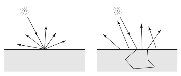
But this assumption doesn’t hold for subsurface scattering which is why we need a more complicated equation that integrates radiance over incoming directions and area, $A$.
$$L_{0}\left(\mathbf{x}, \omega_{0},...\right)=\int_{A} \int_{\Omega} S\left(x_{i}, \omega_{i} ; x_{0}, \omega_{0}\right) L_{i}\left(x_{i}, \omega_{i}\right)\left(n \cdot \omega_{i}\right) d \omega_{i} d A\left(x_{i}\right)$$
Where $S(\cdot)$ is the BSDF which fully describes the material.
While we could use pathtracing to evaluate the modified rendering equation by spawning refraction rays, the paper “A Practical Model for Subsurface Light Transport by Henrik Jensen et.al.” describes a way of approximating our BSDF with a BRDF letting us use our unmodified rendering equation.
By assuming that the incident illumination is uniform, we can integrate the BSDF.
Integrating the diffuse term, we get the diffuse reluctance, $R_d$:
$$R_{d}=2 \pi \int_{0}^{\infty} R_{d}(r) r d r=\frac{\alpha^{\prime}}{2}\left(1+e^{-\frac{4}{3} A \sqrt{3\left(1-\alpha^{\prime}\right)}}\right) e^{-\sqrt{3\left(1-\alpha^{\prime}\right)}}$$
Where $\alpha$ is the albedo, and $A$ is the internal reflection.
The paper gives us the BRDF for a semi-infinite medium:
$$f_{r}^{(1)}\left(x, \omega_{i}, \omega_{0}\right)=\alpha F \frac{p\left(\omega_{i}^{\prime} \cdot \omega_{0}^{\prime}\right)}{\left|n \cdot \omega_{i}^{\prime}\right|+\left|n \cdot \omega_{0}^{\prime}\right|}$$
Where $F$ is the Fresnel term (the answer is too long for explaining the Fresnel equation), $p$ is the phase function - without it the scattering can only be isotropic.
However, we also need to account for the diffuse reflectance, so the complete BRDF becomes:
$$f_{r}\left(x, \omega_{i}, \omega_{0}\right)=f_{r}^{(1)}\left(x, \omega_{i}, \omega_{0}\right)+F \frac{R_d}{\pi}.$$
Implementation
All of this theory gives us the following simple algorithm which can produce images indistinguishable from real photographs given the right parameters.
If that’s not impressive, I don’t know what is.
Color TracePath(Ray ray, count depth) {
    if (depth >= MaxDepth) {
      return Black;  // Bounced enough times.
    }

    ray.FindNearestObject();
    if (ray.hitSomething == false) {
      return Black;  // Nothing was hit.
    }

    Material material = ray.thingHit->material;
    Color emittance = material.emittance;

    // Pick a random direction from here and keep going.
    Ray newRay;
    newRay.origin = ray.pointWhereObjWasHit;

    // This is NOT a cosine-weighted distribution!
    newRay.direction = RandomUnitVectorInHemisphereOf(ray.normalWhereObjWasHit);

    // Probability of the newRay
    const float p = 1/(2*M_PI);

    // Compute the BRDF for this ray (assuming Lambertian reflection)
    float cos_theta = DotProduct(newRay.direction, ray.normalWhereObjWasHit);
    Color BRDF = material.reflectance / M_PI ;

    // Recursively trace reflected light sources.
    Color incoming = TracePath(newRay, depth + 1);

    // Apply the Rendering Equation here.
    return emittance + (BRDF * incoming * cos_theta / p);
  }
(Naive pseudo-code from Wikipedia).
If you're curious about how to implement it for real, I have done exactly that: Building a Pretty Fast Path Tracer in Python from Scratch.

Real or fiction?