Building a Pretty Fast Path Tracer in Python from Scratch

We have previously seen the beautiful mathematical formulation of path tracing. However, we didn't actually implement it. Let us change that.

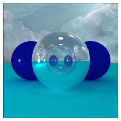
By the end of this walkthrough, we should be able to render images such as this one.

$18_refraction$

However, before we can implement path tracing, we should start simple, and implement a basic ray tracer.

The ray tracer is heavily inspired by Gabriel Gambetta's computer graphics from scratch.

if you just want the code for the path tracer, and don't want the read the whole walkthrough, you can find it on github.

First, we need to set up a canvas we can draw on. Following Gambetta's tutorial, we will have $(0,0)$ in the middle of the canvas, and have $+x$ go to the right, and $+y$ go up.

class Canvas():
    def __init__(self, x, y):
        self.x = x
        self.y = y
        self.pixels = np.zeros((y,x,3),dtype=int)

    def _center2pixel(self, x, y):
        return (self.y//2 - y, self.x//2 + x)

    def write_pixel(self, x, y, color):
        x,y = self._center2pixel(x,y)
        self.pixels[x,y] = color.astype(int)

    def show(self):
        plt.imshow(self.pixels, vmin=0, vmax=255)
        plt.gca().axis('off')
        plt.show()

Next, we will quickly set up a basic camera. We follow the convention common in computer graphics that $z$ follows the camera's direction, and $y$ is up and $x$ is right from the camera's perspective.

class Camera():
    def __init__(self, position=(0,0,0), orientation=[[1,0,0],[0,1,0],[0,0,1]], d=1, w=1, h=1, resolution=(100,100)):
        self.position = np.array(position)
        self.orientation = np.array(orientation)
        # distance from camera to canvas
        self.d = d

        # width and height of camera frame otherwise known as the FoV
        self.w = w
        self.h = h

        self.resolution = resolution

        if not resolution[1]/self.resolution[0] == h/w:
            raise "Resolution does not match aspect ratio"

        self.canvas = Canvas(*resolution)

    def canvas_to_world(self, x, y):
        return (x*self.w/self.resolution[0], y*self.h/self.resolution[1], self.d)

Now that we have the basic functionality in place, it's time to start creating some rays. The basic idea of ray tracing is to shoot rays out of the camera through each pixel (which is why the canvas is projected in front of the camera) until it hits an object.

But before we can do that, we should create a ray class.

class Ray():
    def __init__(self, origin, direction, tmin=1, tmax=np.inf):
        self.origin = np.array(origin)
        self.direction = np.array(direction)

        self.tmin = tmin
        self.tmax = tmax

    def p(self, t):
        return self.origin + t*self.direction

We represent the ray using a point for the origin, and a vector for the direction it goes. We further keep track of the minimum and maximum travel distance for the ray. We don't end up using maximum distance, but when we bounce rays, having a small postive minimum distance prevents it from intersecting with the object it just hit.

The $p$ function simply gives the point of the ray at time $t$.

Next, we need a primitive for which the ray can intersect. For simplicity, we will use a sphere.

class Sphere():
    def __init__(self, position=(0,0,5), radius=1, material=BasicMaterial((255,255,255))):
        self.position = np.array(position)
        self.radius = np.array(radius)
        self.material = material

    def intersect(self, ray):
        a = np.dot(ray.direction, ray.direction)
        b = 2*np.dot(ray.origin-self.position, ray.direction)
        c = np.dot(ray.origin-self.position, ray.origin-self.position) - self.radius**2

        discriminant = b**2 - 4*a*c

        if discriminant < 0:
            return [np.inf]
        else:
            t1 = (-b - np.sqrt(discriminant))/(2*a)
            t2 = (-b + np.sqrt(discriminant))/(2*a)
            return [t1,t2]

    def normal(self, point):
        # return normalized normal vector. 
        return (point-self.position)/self.radius

There are two important functions for the primitive class: The intersection functions that gives a list of times when the ray hits the primitive. In the case of the circle, there will be a single intersection if the ray hits the edge, two intersections if the ray hits the middle, and zero intersections if the ray misses the sphere.

The normal method should return the normal vector at the point of the circle. We won't use it yet, but it becomes very important later.

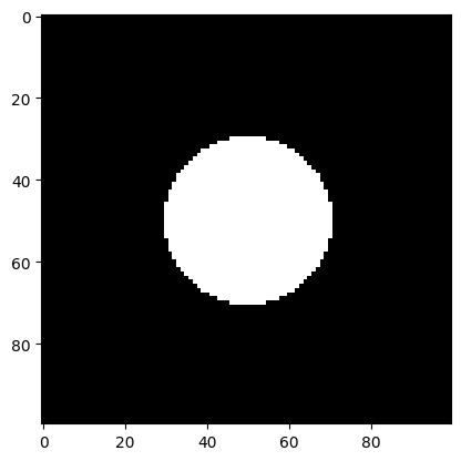
We now have all the ingredients to render a circle if we shoot a ray through each pixel, and if we hit the circle we paint the pixel white otherwise we just paint it black. We should get something like this:

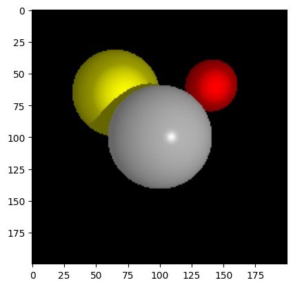
We can also easily extend this to multiple objects with multiple colours. For each object attach a material that has a color.

For each pixel we should now send out a ray and test if it intersects each object the closest of which we paint its color. We may do something like this

def closest_intersection(ray, objects):
    closest_object = None
    closest_t = np.inf
    for obj in objects:
        ts = obj.intersect(ray)
        for t in ts:
            if ray.tmin<=t<=ray.tmax:
                if t<closest_t:
                    closest_object = obj
                    closest_t = t
    return closest_object, closest_t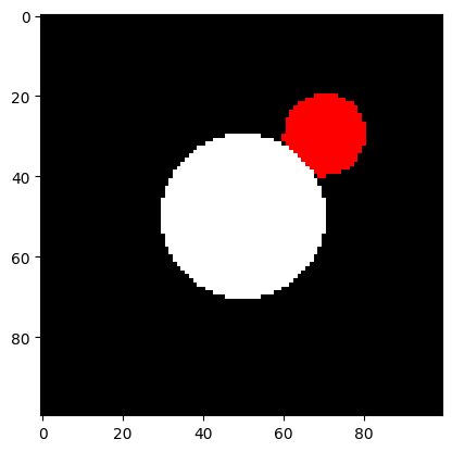

However, in real life, objects are not just one color they have some shading depending on the light direction. Which means we should define some lights.

For simplicity, we will only define a point light without any falloff. For this we just need the light direction vector $L$ from any point in the world as well as the intensity. (We will assume that the color of the light is white)

class PointLight():
    def __init__(self, position, intensity):
        self.position = np.array(position)
        self.intensity = intensity

    def get_L(self, P):
        return self.position - P

Now how do we shade the spheres? We can multiply the light intensity by the cosine of the angle between the light vector and the normal to the intersection point. In code, we might do something like the following

if N_dot_L>0:
     I+= light.intensity * N_dot_L/(np.linalg.norm(L)*np.linalg.norm(N))

Remember the dot product between two vectors is equal to the cosine of the angle multiplied by the lengths.

Moreover, notice that we only add the diffuse light if the dot product is positive to avoid the light darkening the pixel.

Doing this should produce an image like this

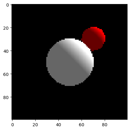
Here we also added an ambient light that is the base color of the sphere when no light hits it to avoid the dark side being completely black. This simulates indirect lighting where light would bounce off the other objects.

This is already much better, but surfaces are not always matte, so we should also add some specular highlights.

Specular highlights, unlike diffuse shading, depend on the view direction $V$. When you move the camera, the specular highlights move along.

Let $R$ be the reflected ray direction. Then the specular highlight is given by $(R\cdot V)^{specular}$ where $specular$ is a some constant that determines how concentrated the highlight is with higher values being more concentrated.

In code you might represent it like so:

if material.specular != 0:
    R = 2*N_dot_L*N - L
    R_dot_V = np.dot(R, V)
    if R_dot_V>0:
        I+= light.intensity * np.power(R_dot_V/(np.linalg.norm(R)*np.linalg.norm(V)), material.specular)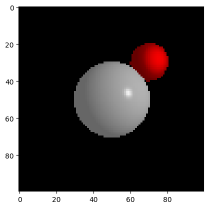

This light model is pretty close to the Phong model. However, we still need some features for us to be happy with our light transport.

In particular we need shadows.

The way we get shadows is by after having found the intersection point for the ray, we loop through all the lights and cast a ray from the point to the light to ask if the view is unobstructed. If the view is obstructed by another object, we paint the object in shadow that is only the ambient light color is rendered.

In code this might look like

def is_in_shadow(self, P, light, closest_object):
    L = light.get_L(P)
    ray = Ray(P, L, tmin=0.001, tmax=np.inf)

    closest_object, closest_t = closest_intersection(ray, self.objects)
    
    if closest_object is None:
        shadow = False
    else:
        shadow = True

    return shadow

If implemented correctly, we should get shadows like the below.

Notice that the shadows are hard shadows. This comes from the light source being a point light instead of a light with a surface area. We will address this issue when we extend the ray tracer to become a path tracer.

But there is one last thing we need. We need reflections.

Reflections work much the same way as we computed the specular highlights. We simply compute the reflected direction and send out a new ray going in the reflected direction from the intersection point and compute its color.

Then we mix the local color and the reflected color to get the final color according to how reflective the material is.

local_color * (1- r) + r * reflected_color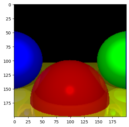

This marks the end of the ray tracer, there is only one thing left and that is to add a background skybox to make the reflections more interesting.

We do this by taking a cubemap and projecting it into a sphere, then if we don't hit an object, instead of just returning a black color, we return the color of the texture at the point on the big projected sphere we necessarily hit.

We should get something like this.

Before moving on to path tracing, you should checkout the full ray tracer.

Path Tracing

The basic differences between ray tracing and path tracing are:

Path tracing is stochastic, we sample many rays per pixel
Path tracing does not trace explicit shadow or reflection rays, we just bounce rays in the scene until we hit our recursion limit.
Path tracing doesn't work with point lights.
Path tracing can produce more realistic lighting including global illumination.
Path tracing is much more expensive.

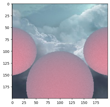
If we just sample multiple rays per pixel in our current ray tracer, we get the code here, and the following output.

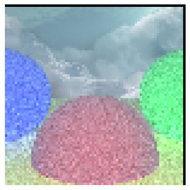
However, our code is not very optimised which is why we are not able to run many samples per pixel, and why we see a lot of noise.

If we, however, optimise the code using Numba, we can get much higher samples per pixel.

Now, we need to simplify how we do light transport. Instead of bouncing explicit shadow and light rays, we should just send out rays and hope we hit some light source.

But how do we determine which kind of bounce we do. Simple, we just sample the kind of bounce according to the probabilities defined by the material. So currently, we can do reflection, specular, or diffusion

For reflection and specular we should sample the direction in a cone around the reflected direction. However, I currently only implement perfect reflection where it will always go in the direction of the perfect reflection.

Diffusion bounces, on the other hand, will always sample uniformly from the hemisphere above the surface normal.

This new light transport looks like this

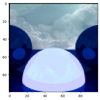
Not the prettiest, but that's because we haven't tweaked the values yet, and the middle sphere is emitting light.

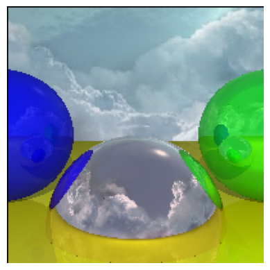
The final thing we want to add is refraction where light travels through the material and is bend according the the refractive index of the material.

Here we should obey the Fresnel equations, but because it's computationally more efficient, we will use Schlick's approximation.

When implemented, we can get images like the first image shown.

$18_refraction$

Here is where the walkthrough ends. However, I did work on a couple of more features that I wasn't able to figure out.

The first feature is caustics. I thought caustics would come for free when you implement refractions correctly, however, I haven't been able to observe caustics in any of my renders.

I thought perhaps I implemented it wrongly, so I borrowed someone else's code and integrated it into my rendering pipeline, but still wasn't able to observe any caustics.

I know that backwards path tracing (where we shoot rays from the camera) is terribly inefficient at rendering caustics, and we should ideally be using bi-directional path tracing, or photon mapping to get caustics. However, I have seen renders using backwards path tracing get noisy caustics, so the fact that I get nothing puzzles me.

Really, if you have any insight, please contact me.

The other feature was implementing arbitrary meshes which I did get to work, but was terribly slow, so I tried to speed it up by constructing a kd-tree for the triangles. However, something is wrong with my implementation of the kd-tree traversal. It doesn't make it easier that I'm not able to have class inheritance or composition with numba, so I have to represent the tree as an array.

I might return to this some day as it bugs me that I didn't quite reach my goals, but for now this is a pretty fast path tracer implemented from scratch in python.

By Luna Lux Fredenslund